Binomial Puzzles: Warwick Statistics Department Puzzle

The Puzzle

My Solution

So, we are told that we have n fair coins and we flip them. We remove those that landed tails and flip again the heads. We need to give the distribution of the number of heads after this second round. This means that if we denote as X the number of coins we would flip in the second round and H the number of final heads we have: X∼Bin(n,p=0.5) and H|X=x∼Bin(x,p=0.5),

we are asked about the unconditional distribution of H.

However we can rephrase the problem as follows:

1. Flip each of the n fair coins twice
2. Call it a success whenever both flips are heads.
3. What is the distribution of the number of succesesses?

This is equivalent, but it makes the solution apparent. We are being asked about another Binomial distribution, just that now the probability of success is that of having two heads in two consecutive independent fair coin tosses; which is just 0.5(0.5)=0.25. Hence, H∼Bin(n,p=0.25).

If you are still not convinced, let’s provide a mathematical proof. In fact, we can even generalize this problem by not requiring the tosses to be fair or even have the same probability in both rounds. The more general result is that H∼Bin(n,p=p1p2),

where pi is the probability of heads in the i-th round.

Indeed, P(H=h)=n∑x=0P(H=h|X=x)P(X=x)=n∑x=h(xh)ph2(1−p2)x−h(nx)px1(1−p1)n−x=n∑x=h(nh)(n−hx−h)ph2(1−p2)x−hpx1(1−p1)n−x=(nh)n−h∑k=0(n−hk)ph2(1−p2)(k+h)−hpk+h1(1−p1)n−(k+h)=(nh)(p1p2)hn−h∑k=0(n−hk)[p1(1−p2)]k(1−p1)(n−h)−k=(nh)(p1p2)h[p1(1−p2)+(1−p1)]n−h=(nh)(p1p2)h(1−p1p2)n−h,

where we used a change of variable k=x−h and the second to last step follows from the Binomial Theorem. We recognize this last expression as the probability mass function of a Binomial random variable with paramenters n and p=p1p2, as claimed.

Bonus Question

As for the Bonus question, it is also an interesting exercise. If we start with n=1600 fair coins and at each turn we eliminate those landing tails, we wonder, how many rounds on average we will have before running out of coins.

A first approximation would be to say that, on average, we would expect to lose half of the coins each time. After the first toss we will end up with around 800, then 400, and after 6 round we would expect to have only around 25 coins. Now we are expecting to have an odd number of coins but we could keep halving until we have close to a single coin. That is, after 10 rounds, 1600210≈1.5625 and so that we may expect to have at least an eleventh round before running out of coins. But, is the answer then 11, 12, 13,…?

Just like with the main puzzle, by rephrasing the problem in terms of flipping all the n coins and just considering a different notion of success we can come up with a better solution. Let us focus on a single coin; we would keep flipping it as long as it keeps turning heads. Well, the number of times we will flip said coin can be modeled as a Geometric random variable where now the success is landing tails. We see then that we will run out of coins the last time where a given coin lands tails for the first time. This is just to say that we are interested in the maximum of a series of n independent Geometric random variables with parameter p=0.5 or, more precisely, in its expected value.

Mathematically, let us denote as X the number of flips of a coin before observing the first tail. Then X∼Geo(p), where we are now generalizing and not limiting ourselves to the case of equiprobability; although, contrary to the main puzzle, here we do keep assuming that the probability of tails in each round remains the same. Then τ:=max{X1,X2,…,Xn}∼Fτ,

where, Fτ(t)=P(τ≤t)=[P(X≤t)]n=[1−(1−p)t]n.

We can then use the survival form of the expectation to have the following expression: E[τ]=∞∑t=0P(τ>t)=∞∑t=01−[1−qt]n,

where q=1−p is the probability of heads. Now, without being a formal proof, we see that this sum will converge since the terms will go relatively quickly to 0 as t grows. This allows us to propose an R function that approximates the sum for us:

ev_max_geo <- function(n, q, max_iter = 1000, tol = 1e-10){
  
  ev_tau <- 0
  s_t <- tol + 3
  t <- 0
  while(s_t > tol && t <= max_iter){
    s_t <- 1 - (1-q^t)^n
    ev_tau <- ev_tau + s_t
    t <- t + 1
  }
  
  return(ev_tau)
  
}

ev_max_geo(n = 1600, q = 0.5)

## [1] 11.97705

The solution is, rounding, 12!

We can go a little bit further with R and verify via Monte Carlo that this is correct. We can simulate 10,000 experiments each starting with 1600 coins

ruin_exp <- function(n, q, max_k = 1e5){
  
  k <- 0
  
  while(n > 0 && k <= max_k){
    n <- rbinom(1, size = n, prob = q)
    k <- k + 1
  }
  
  return(k)
  
}

set.seed(220206)
tau <- rep(NA, 10000)
for(i in seq_along(tau)){
  tau[i] <- ruin_exp(n = 1600, q = 0.5)
}

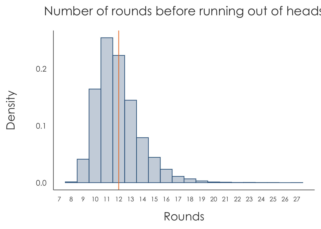
summary(tau)

##    Min. 1st Qu.  Median    Mean 3rd Qu.    Max. 
##    8.00   11.00   12.00   11.96   13.00   27.00

In fact, we have the following approximation to the distribution of τ:

library(ggplot2)
library(fazhthemes)

hist_tau <- ggplot(data = data.frame(tau = tau), 
                   aes(x = tau, y=..density..)) + 
  geom_histogram(fill = "steelblue4", color = "steelblue4", 
                 alpha = 0.3, binwidth = 1, center = 0) + 
  geom_vline(xintercept = 12, color = "chocolate2") + 
  labs(x = "Rounds", y = "Density", 
       title = "Number of rounds before running out of heads", 
       subtilte = "starting with 1600 fair coins") + 
  scale_x_continuous(breaks = 0:max(tau)) + 
  lucify_theme_classic()

plot(hist_tau)